Here at FullContact we have lots and lots of contact data. In
particular we have more than a billion profiles over which we would like
to perform ad hoc data analysis. Much of this data resides in Cassandra, and we have many analytics jobs that require us to iterate across terabytes of data within this Cassandra data.
Using Netflix Priam makes the Cassandra backup process a snap, and so we were able to bring up a backup Cassandra cluster fairly easily. With the backup cluster in place we could do whatever analysis was needed by querying Cassandra directly from MapReduce jobs.
But while the process worked, there were still drawbacks – our data analysis jobs were slow. We were still limited by query rates maxing out at around 1000 QPS to Cassandra, which restricted how fast we could process data on a MapReduce cluster. In order to process the quantity of data we had, the MapReduce jobs took anywhere from 3-10 days. Getting results was taking way too long – not to mention how painful it was if you found you were missing something crucial in the final result.
Iterating with these kinds of turnaround times didn’t scale.
So we set out hoping to find and leverage an existing solution. In the end we rolled our own solution which will be open sourced in the near future. This is the story of our journey – let the spelunking begin!
As I mentioned, we use Netflix Priam to manage our Cassandra backups. Priam stores the SSTable files on S3 for offline storage. If we could leverage these SSTable files directly, then we would be able to process the Cassandra data on MapReduce. Having a similar requirement, Netflix developed Aegisthus which appeared to do exactly what we needed: Aegisthus processes the SSTables from the Priam backups directly on MapReduce. We were pretty excited to try out Aegisthus for our use case.
Initially, Aegisthus looked promising. The idea was to transfer the Priam backup from S3 to HDFS and then process them with Aegisthus. However, we ran into a few snags along the way.
First I should mention that Priam snappy compresses the backup files while they are streamed to S3. However, Aegisthus assumes that the files have already been decompressed. Because of this, we needed to preprocess the Priam backups while streaming them from S3. We developed a custom distributed copy which decompresses the snappy files in-flight. We needed this because Priam compresses files with snappy-java which is not supported by the snappy compression supplied with Hadoop. There are currently several implementations of snappy which are not all compatible – in this case we’re dealing with both java-snappy and hadoop snappy. With this in place, we were ready to process our SSTables with Aegisthus.
The next issue we ran into was support for our version of Cassandra. We are currently on Cassandra 1.2 and the initial release of Aegisthus only supported Cassandra 1.1. Fortunately the guys over at Coursera had an experimental branch going with support for Cassandra 1.2. We gave this a try on a small sample of SSTable data and initial results looked good; we were excited to try it on our entire cluster.
KassandraMRHelper has the same goal of allowing for offline processing of Cassandra data by leveraging the SSTables from a Priam backup. Additionally, they handle snappy decompressing of the Priam backup on the fly. Cool, we were excited to give this a shot. Unfortunately we ran into a few snags here as well.
First, KassandraMRHelper used Cassandra’s I/O code to handle reading the SSTables which required that the SSTables be copied to the local file system because Cassandra’s I/O code did not support HDFS. This was problematic for us with individual SSTables on the order of 200 GB and a 4.5 TB cluster size. The snappy decompression was done on the local file system, as well, prior to reading the SSTables. This required decompressing a 200 GB file which resulted in more than doubling the storage capacity requirements.
This didn’t work for us as we would continually run out of disk space during the decompression phase. To get around this, we leveraged our custom distributed copy to decompress the Priam backups as they were streamed to HDFS from S3 and disabled the decompression code in KassandraMRHelper. This gave us the headroom to process our files, but we were still left with some issues:
At this point we had accomplished our first goal. We were able to perform the data analysis we needed by leveraging the SSTables from our Priam backups. However, we still needed better performance. To get there we needed to be able to scale horizontally, so we decided it was worth it to roll our own splittable SSTable input format for Cassandra SSTables.
We decided to implement the splittable SSTable input format using a similar approach as the splittable LZO input format implementation. We chose this because there are some similar aspects between the two. In both LZO and SSTable files there are compressed blocks which can be read independently and in a random access fashion. Also, we can generate an index for both by preprocessing the files themselves. Generating the index before reading the SSTable files, similar to LZO, saved us 18 hours of processing time in our test case. We were able to build the SSTable index by leveraging some of the metadata that comes along with each SSTable.
Each Cassandra SSTable is made up of several files. For our purposes we really only care about three of them:
Slow Going
Unfortunately, support for performing this kind of data analysis with Cassandra is limited. When we began working on the data analysis problem, we understood that because we use MapReduce, we would be forced to perform live queries to Cassandra – bad news. So in order to obviate the performance concerns on our already heavily loaded Cassandra clusters, we realized that performing these ad hoc analytic jobs had to be executed against an entirely isolated ‘backup’ cluster.Using Netflix Priam makes the Cassandra backup process a snap, and so we were able to bring up a backup Cassandra cluster fairly easily. With the backup cluster in place we could do whatever analysis was needed by querying Cassandra directly from MapReduce jobs.
But while the process worked, there were still drawbacks – our data analysis jobs were slow. We were still limited by query rates maxing out at around 1000 QPS to Cassandra, which restricted how fast we could process data on a MapReduce cluster. In order to process the quantity of data we had, the MapReduce jobs took anywhere from 3-10 days. Getting results was taking way too long – not to mention how painful it was if you found you were missing something crucial in the final result.
Iterating with these kinds of turnaround times didn’t scale.
So we set out hoping to find and leverage an existing solution. In the end we rolled our own solution which will be open sourced in the near future. This is the story of our journey – let the spelunking begin!
Background
It was clear that querying Cassandra directly wasn’t going to scale for our application. We needed to be able to access the data directly for our MapReduce jobs to perform. The best solution for this would be to have the data available directly on HDFS (Hadoop Distributed File System). Fortunately Cassandra stores all of its data directly on the file system in sorted string format or SSTable format. Because the data in these files are already sorted by key, they are ideal for processing with MapReduce. With this in mind we set out to process the SSTables directly.As I mentioned, we use Netflix Priam to manage our Cassandra backups. Priam stores the SSTable files on S3 for offline storage. If we could leverage these SSTable files directly, then we would be able to process the Cassandra data on MapReduce. Having a similar requirement, Netflix developed Aegisthus which appeared to do exactly what we needed: Aegisthus processes the SSTables from the Priam backups directly on MapReduce. We were pretty excited to try out Aegisthus for our use case.
Initially, Aegisthus looked promising. The idea was to transfer the Priam backup from S3 to HDFS and then process them with Aegisthus. However, we ran into a few snags along the way.
First I should mention that Priam snappy compresses the backup files while they are streamed to S3. However, Aegisthus assumes that the files have already been decompressed. Because of this, we needed to preprocess the Priam backups while streaming them from S3. We developed a custom distributed copy which decompresses the snappy files in-flight. We needed this because Priam compresses files with snappy-java which is not supported by the snappy compression supplied with Hadoop. There are currently several implementations of snappy which are not all compatible – in this case we’re dealing with both java-snappy and hadoop snappy. With this in place, we were ready to process our SSTables with Aegisthus.
The next issue we ran into was support for our version of Cassandra. We are currently on Cassandra 1.2 and the initial release of Aegisthus only supported Cassandra 1.1. Fortunately the guys over at Coursera had an experimental branch going with support for Cassandra 1.2. We gave this a try on a small sample of SSTable data and initial results looked good; we were excited to try it on our entire cluster.
As it turns out, Netflix had a slightly different use case
than ours and Aegisthus was built to support that use case well. Here
are the main differences:
- SSTable compression: Aegisthus does not support splitting of SSTables with compression enabled, only SSTables that are uncompressed. Thus, the reason Priam snappy compresses the backup files. This didn’t add a lot of value for us since we do enable compression on the Cassandra SSTables—we ended up with SSTables which were essentially double snappy compressed. We needed a solution that supported splitting SSTables which have compression enabled.
- Cassandra version: We used Cassandra 1.2 while Aegisthus only supported Cassandra 1.1 at the time.
- Compaction Strategy: We used size tiered compaction which resulted in very large SSTables which are not splittable.
KassandraMRHelper has the same goal of allowing for offline processing of Cassandra data by leveraging the SSTables from a Priam backup. Additionally, they handle snappy decompressing of the Priam backup on the fly. Cool, we were excited to give this a shot. Unfortunately we ran into a few snags here as well.
First, KassandraMRHelper used Cassandra’s I/O code to handle reading the SSTables which required that the SSTables be copied to the local file system because Cassandra’s I/O code did not support HDFS. This was problematic for us with individual SSTables on the order of 200 GB and a 4.5 TB cluster size. The snappy decompression was done on the local file system, as well, prior to reading the SSTables. This required decompressing a 200 GB file which resulted in more than doubling the storage capacity requirements.
This didn’t work for us as we would continually run out of disk space during the decompression phase. To get around this, we leveraged our custom distributed copy to decompress the Priam backups as they were streamed to HDFS from S3 and disabled the decompression code in KassandraMRHelper. This gave us the headroom to process our files, but we were still left with some issues:
- KassandraMRHelper still copied the SSTables to the local file system to be read with Cassandra I/O code.
- KassandraMRHelper’s SSTable input format is not splittable.
At this point we had accomplished our first goal. We were able to perform the data analysis we needed by leveraging the SSTables from our Priam backups. However, we still needed better performance. To get there we needed to be able to scale horizontally, so we decided it was worth it to roll our own splittable SSTable input format for Cassandra SSTables.
Implementing a Splittable Input Format
Our approach to implementing a splittable SSTable input format came after a lot of exploration for existing implementations. In the end we borrowed some of the best ideas from the solutions we tried and rolled them into a generic input format which can read any Cassandra SSTable in a splittable fashion. This allows us to properly leverage MapReduce for what it’s good at—parallel processing large amounts of data.We decided to implement the splittable SSTable input format using a similar approach as the splittable LZO input format implementation. We chose this because there are some similar aspects between the two. In both LZO and SSTable files there are compressed blocks which can be read independently and in a random access fashion. Also, we can generate an index for both by preprocessing the files themselves. Generating the index before reading the SSTable files, similar to LZO, saved us 18 hours of processing time in our test case. We were able to build the SSTable index by leveraging some of the metadata that comes along with each SSTable.
Each Cassandra SSTable is made up of several files. For our purposes we really only care about three of them:
- Data file: This file contains the actual SSTable data. A binary format of key/value row data.
- Index file: This file contains an index into the data file for each row key.
- CompressionInfo file: This file contains an index into the data file for each compressed block. This file is available when compression has been enabled for a Cassandra column family.
Cassandra’s I/O code handles random access into the
compressed data seamlessly by leveraging the CompressionInfo file for
the corresponding Data file. Porting this code to work with HDFS allows
us to read the SSTable in the same random access fashion directly within
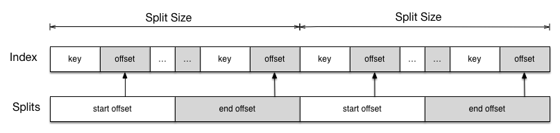
MapReduce. The Index file allows us to define splits as we see fit.
Using both of these together allowed us to define an input
format which can split the SSTable file and distribute those splits. The
downside is that we will have to add support for new versions of
Cassandra as the SSTable file format changes, but this is acceptable to
get the results that we need.
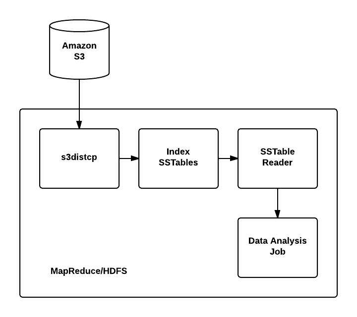
The final pipeline is detailed in the diagram below.
The first step in our pipeline is a transfer of the Priam
backup from S3 to HDFS. The Priam backup files themselves are
decompressed inline during this step. Next we index the SSTables which
essentially defines the splits which will be used by the input format.
Split size can be tuned as needed for a particular application. After
indexing the SSTables we can process them using the SSTable input
format. The best part of implementing this as an input format is that we
can write any number of MapReduce jobs to process that data in whatever
way we like.
For us, we use the SSTable reader step to build
intermediate data that feeds downstream jobs. The SSTable input format
reads the split information from the index step. The SSTable record
reader reads records by seeking to start of the split and reading
SSTable row records sequentially to the end of the split. A best guess
is made as to which MapReduce node the split should be processed on for
data locality. This guess is based on the compressed file size as we do
not have the compression metadata (CompresssionInfo) that contains the
uncompressed file size at the time of split calculation and reading that
metadata is expensive enough to avoid it where we can.
Now that we’ve successfully read the SSTables and have an
acceptable intermediate data format we’re free to run whatever data
analysis jobs we like across the data. Currently we are leveraging JSON
as the intermediate data format, but we have plans to use a more compact
format in the future.
Results
Reading Cassandra SSTables has become scalable and
performant with this new input format. For each of our tests we ran an
Amazon Elastic MapReduce cluster consisting of 20 m2.4xlarge nodes. In
all cases, we processed an entire Cassandra cluster’s data approximately
4.5 TB in size. The results are summarized in the table below.
Cassandra Data Processing Results
|
|
Reading via live queries to Cassandra
|
3-10 days
|
Unsplittable SSTable input format
|
60 hours
|
Splittable SSTable input format
|
10 hours
|
After implementing the splittable SSTable input
format we’ve been able to reduce our processing time from 3-10 days to
under 10 hours on a baseline 20 node MapReduce cluster. It is
worth noting that these results are achieved with little or no tuning.
Currently, the map phase of our reader job is CPU bound while the reduce
phase is I/O bound. We believe this will become progressively faster as
we continue to tune MapReduce and the split sizes to optimize cluster
performance.
Where We’re Going
The best part about having this new input format available
to process Cassandra data offline in a reasonable amount of time is that
it opens the door to doing all sorts of analytics on our Cassandra
data. There are many applications outside of the single use case we’ve
outlined here, and we hope that others will benefit from its usefulness
as well. Which is why we are excited to open source the splittable
SSTable input format in the coming weeks.


No comments:
Post a Comment